How carbon dating works

by Robert W. Carter

Background

“What about carbon dating?” is a question our speakers are often asked after giving a creation presentation at a church. In fact, it is such a common question that we included an entire chapter about it in our Creation Answers Book. We have written about how carbon dating of ‘ancient’ things like diamonds is a strong indication that earth is young and how carbon dating of tree rings challenges (unsuccessfully, mind you) biblical chronology. Yet, people are still confused about carbon dating, so we decided to put everything into one place. Below, you will find an explanation of what carbon dating is, how the tests are done, and how it impacts our understanding of the Bible.

Many people use ‘carbon dating’ as shorthand for all radiometric dating techniques. One of my favorite questions to ask after getting the inevitable carbon dating question is, “Excuse me, do you mean ‘carbon dating’ or radiometric dating in general, like uranium to lead or potassium-40 to argon-40?” The look on their face is usually one of confusion as the questioner suddenly realizes they did not even realize what they were asking. Each of the other techniques has its own answers, but as far as carbon dating is concerned, it is a wonderful tool for biblical creationists. It gives us solid evidence that the earth is young (if we can really call such a great age as ~6,000 years “young”). Before we draw that conclusion, however, we have a few things to learn.

Radioactive decay rates and half-life

Carbon-14 cannot be used to date very ancient things. As Dr Jonathan Sarfati pointed out in our documentary Evolution’s Achilles’ Heels, if the entire earth were composed of carbon-14, it would completely vanish in less than a million years.

To understand why, one needs to understand the concept of a half-life. This is simply the amount of time it takes for ½ of a radioactive material to break down. If the earth were a giant ball of pure carbon-14, after only one half-life (5,700 ± 30 years) fully one-half of all the atoms would have already decayed (into nitrogen-14 atoms). After less than 12,000 years, only ¼ of the earth would remain. There are about 1×10⁵⁰ atoms within our planet. If, instead of being mostly iron, these were all carbon-14, and if half of those disappear every 5,700 years, there would not be a single carbon-14 atom left before one million years had passed.¹ For this reason, carbon dating can only be used on recent material, and it cannot be used for estimating ages in the millions- or billions-of-years range. So, no, carbon dating does not prove the earth is old. For answers to other radiometric dating techniques, see our Radiometric Dating Questions and Answers page.

The invention of carbon dating

The carbon dating technique was invented by the American scientist Willard Libby in the 1940s. He received the 1960 Nobel Prize in Chemistry for his pioneering work. Modern carbon dating does not use his original method, but it is worth describing. Essentially, by placing a carbon sample in a radiation-shielded box, you can use a scintillation counter to measure the decay of carbon-14 atoms in the sample. Most people are familiar with the hand-held Geiger counter and its characteristic ‘clicking’ sound. This is a scintillation counter. Libby’s method involved counting the beta particles (high energy electrons) emanating from a sample of carbon as the carbon-14 in it decayed into nitrogen-14.

Since carbon-14 has a short half-life, the amount of carbon-14 in a sample should diminish rapidly. For example, a sample from 3,700 BC (one half-life ago) should have about half the carbon-14 as a sample from the modern era. At least in theory, for as we shall see, there are multiple issues with a date like this. For starters, that would place the sample before Noah’s Flood!

As expected, Libby found that younger samples produced more beta particles than older samples, and by correlating the numbers with samples of known age, he could make an educated guess about the age of undated samples. Today, most carbon dating laboratories use an accelerator mass spectrometer (AMS), which will be described below. These came into popular use in the 1980s (figure 1).²

Biblical implications

This discovery had immediate and strong implications for Bible believers. Libby published the first carbon-14 dates for historical artifacts in 1949, and they seemed to invalidate the biblical timeline. He dated sarcophagus lids from the tombs of Djoser (the first pharaoh of Egypt’s 3^rd Dynasty) and Sneferu (the first pharaoh of Egypt’s 4^th Dynasty).³ They were ‘carbon dated’ to 2,800 BC ± 250 years. Clearly, the pyramids could not have been built before the Flood. Something was wrong. Later work re-dated the Egyptian pre-dynastic period, using carbon dating to move it forward by over 400 years,⁴ but this was not nearly enough.

In the 1950s, Kathleen Kenyon used the newly invented technique to date the destruction layer at Jericho. She concluded that Jericho was not destroyed by the Israelites. The carbon dates placed the destruction several centuries prior to the Exodus. Of course, academics argue strenuously about the date of the Exodus, and these early carbon dates would be skewed by the lingering effects of the biblical Flood and by earth’s weakening magnetic field (discussed below), so perhaps Kenyon went too far out on a limb. Yet, the seeds for doubting biblical history were sown. They would germinate quickly as the last vestiges of biblical thought were stripped from the field of archaeology.

If you were to stop here, and many do, you would conclude that carbon dating invalidates the biblical timeline of history. However, this would be a gross error. Understood correctly, and when a biblical timeline is applied,carbon dating is great evidence that the earth is not millions of years old. Can we now use it to show that the earth is as young as the Bible claims? Absolutely!

Is carbon dating accurate?

Generally, carbon dating is very accurate. We get consistent results and can often place an artifact into its proper historical context, plus or minus a few years, a few decades, or a few centuries, depending on the age of the sample. Thus, the question is not about the accuracy of the machines but about the assumptions behind the techniques. Our questions concern the oldest samples, not the more recent ones. In fact, carbon dating works very well on objects from the past 2,000 years.

How are the dates obtained?

The science of carbon dating depends on a standardized calibration curve. This is often made by comparing carbon dates for tree rings. Yet, there are several time periods where the curve is essentially flat, meaning the ‘date’ could fall within a range of values. In other places, the calibration line wiggles up and down, meaning a ‘date’ could be any of several possible values. This does not affect the overall conclusion that older samples have less carbon-14 than younger samples, but it does let us know the state of the art.

There are no historical artifacts that can be precisely dated beyond a few thousand years before Christ, and even then, archaeologists argue strenuously about the exact date for many of these. There are, however, physical and biological records that can be used. Specifically, even if no actual tree has lived for tens of thousands of years, tree rings (figure 2) can be correlated from one dead tree to another. Using this statistical approach, scientists have built a putative historical record going back about ~13,000 years.

commons.wikimedia.org

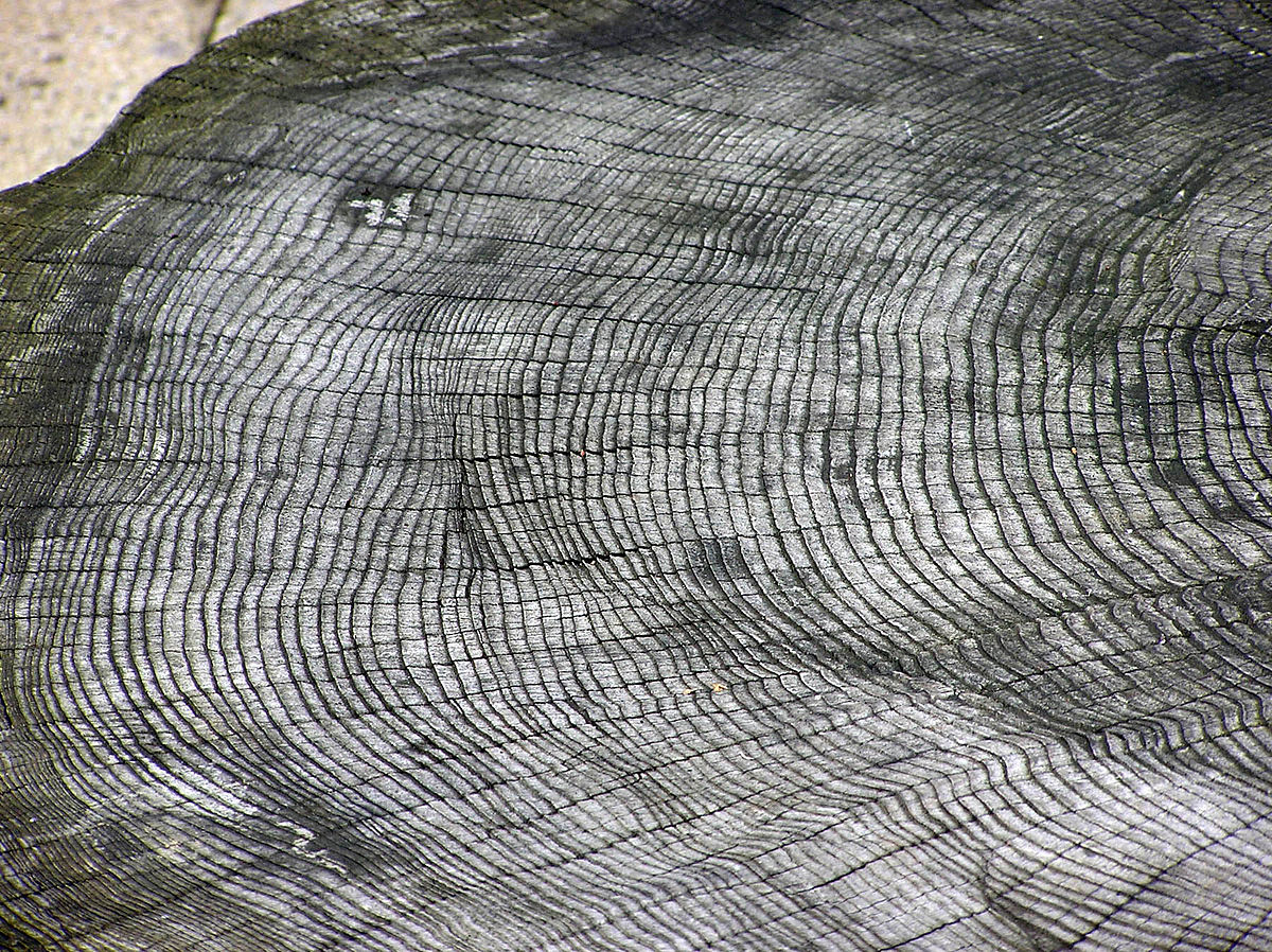
The science of deducing history from tree rings is called dendrochronology, but this is not as straightforward as many believe. First, bristlecone pines can lay down more than one ring per year. Living in the marginal environment of the White Mountains of California, the trees tend to grow whenever the weather conditions are optimal. Also, there is not one, single tree that gives us a complete date range. Instead, the rings from living and dead trees are compared with statistical measures to give ‘best fit’ approximations. This is even true of the highly esteemed Irish oak tree ring record, which was created from trees found in bogs, archaeological wood samples, and beams found in old buildings. The Dendrochronology Laboratory at Queen’s University Belfast has kindly made all their data publicly available so that anyone could build their own dendrochronology. On the data portal page, they wrote:

“Doing so involves making decisions about which ring patterns to include, and is thus an intellectual exercise. Other solutions may exist from the same basic collection of ring patterns, depending on choices made by the analyst, which can then be interpreted as seen fit.”⁵

Being that the tree ring record is such a critical tool for carbon dating ancient artefacts, this is an important consideration. Another problem is that tree ring alignments from locations as close as Northern Ireland, southwest England, and southern Germany disagree strongly.

Likewise, they can use the density bands in dead coral skeletons (figure 3) to model historical changes in carbon-14, but due to the marine reservoir effect and isotopic fractionation (both phenomena are described below), this is problematic. Additional historical and physical models must be applied to the results of any carbon-14 measurement to obtain an estimated date. Also, coral growth can be quite irregular. If you take a core out of any particular colony, you might encounter periods of die back and re-growth or times when one lobe of the colony had overgrown another. In the end, to build a long-term record of coral banding, scientists are forced to correlate the bands from multiple colonies, many of which died a long time ago. This is identical to the situation with tree rings. One cannot simply ‘date’ a coral skeleton.

A third measure involves the thin mud layers (called varves) that form at the bottom of certain lakes. We can question if these are truly annual bands, but there is no question that there are many thousands of varves in places like Lake Suigetsu in Japan (figure 4). This is a shallow lake with an outlet that leads to another lake that is then connected to the ocean. Only very fine silty particles make it into the lake, which then settle out seasonally. And even if the annual bands are not always possible to distinguish, multiple cores have been taken and the banding patterns matched across the cores. This has allowed scientists to (theoretically) piece together a timeline of about 70,000 annual layers. By carbon dating organic material (e.g., leaves) trapped between the layers, they can estimate how much carbon-14 was in the air at specific points in time. They can also see evidence of historic earthquakes (which disturb and mix the surface layers and bring in more sediment than average), periodic floods (which deposit thicker bands), volcanic eruptions (which deposit ash), and westerly winds (which blow in yellow dust from the Gobi Desert of China in the fall and winter months).

commons.wikimedia.org, Phonon.b

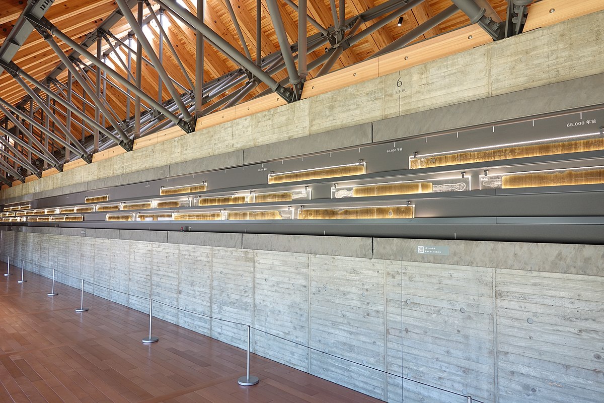
Note, however, that this depends on a very specific set of parameters. The modern lake is only 34 m (111 ft) deep. There are 45 m of well-developed varves and an additional 30 m of mostly non-varved mud beneath that. Even at an estimated deposition rate of 0.7 mm per year, the lake floor must have subsided in reference to the surrounding hills to keep apace of sediment buildup, all while not affecting water influx from the shallow channels that connect the five neighboring lakes. The bottom of the lake also must have remained anoxic for all these thousands of years (this prevents the organic material [leaves] from being consumed by decomposing organisms). Note also that a sediment core does not reveal the horizontal extent of any specific layer. Not only do we not know if these are annual layers, we also do not actually know if each varve spans the whole lake.

Using tree rings, corals banding, and lake varves, the new IntCal20 calibration currently stretches carbon dating back to about 70,000 theoretical years.

Once one has a standardized calibration curve, you can take the results from a carbon-dating test and compare it to known values (figure 5). There are some places where these calibration curves produce nice, clean, unambiguous carbon dates. However, there are other places that are much more difficult to interpret, including some areas where the line wiggles up and down, meaning any object could be assigned any of several possible dates.

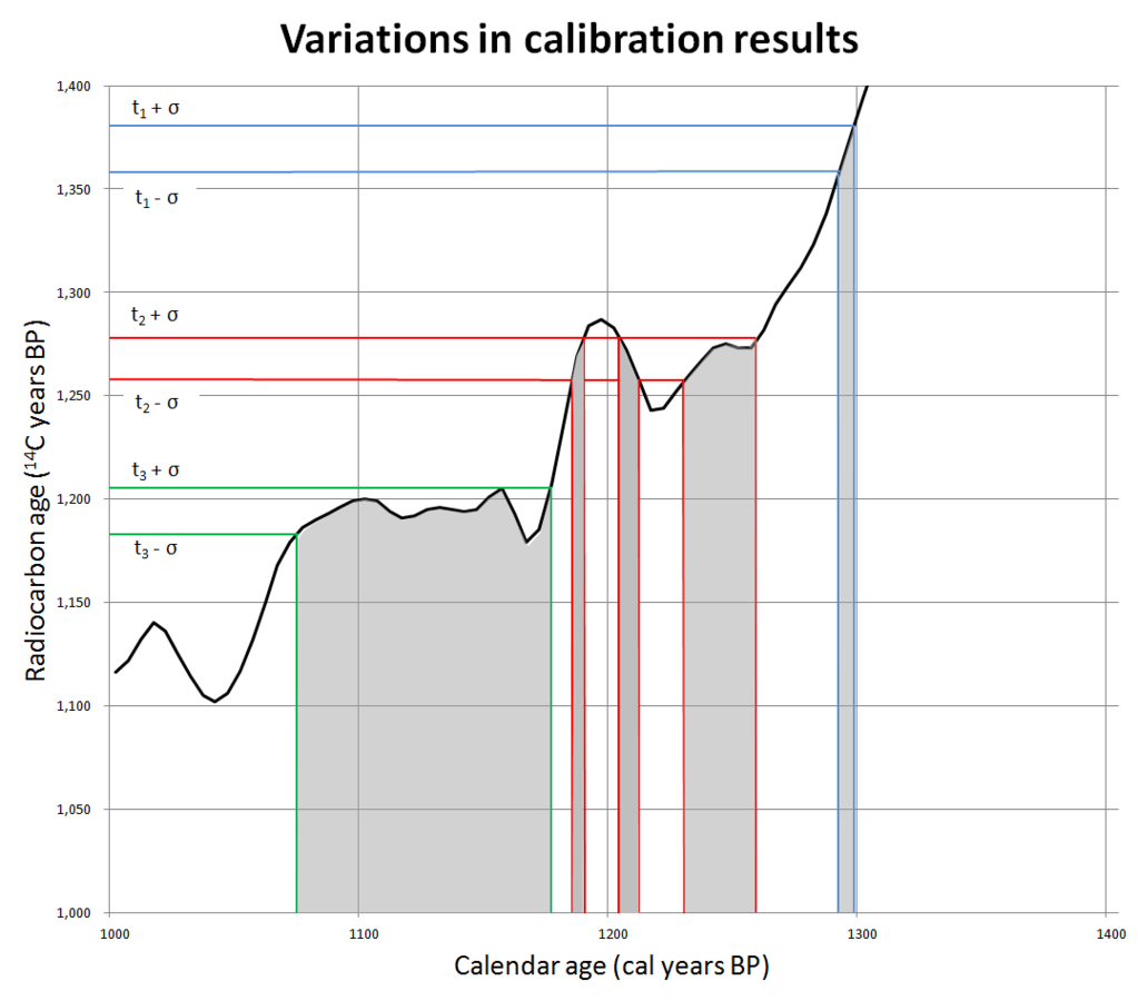
In other places, the curve is flat for decades, sometimes centuries. For example, the timespan from 800 to 400 BC has been called the “Hallstatt plateau” or the “1^st millennium radiocarbon disaster area”. It is a flat spot on the calibration curve that spans a very important time in history. In biblical archaeology, this includes the end of the Divided Monarchy, the fall of Jerusalem, and the Babylonian captivity. The Assyrian, neo-Babylonian, and Persian empires and some of the most important events in Greek antiquity are a carbon-dating cypher. None of these events can be currently resolved with carbon dating! Archaeologists are working hard to fix these issues, but this has been a difficult nut to crack.

Carbon dating is affected by the strength of earth’s magnetic field

There are two historical problems with carbon dating that are generally ignored by secularist scientists and archaeologists. The first is that the earth’s magnetic field is measurably weakening over time. In fact, it is weakening exponentially, by about 5% per century. This gives an upper limit to the age of the earth because the earth does not have an internal power source. The earth itself is not a magnet, because the internal temperature is above the Curie point (the temperature at which magnetism breaks down in a solid metal). Instead, the planet’s magnetism is thought to emanate from circulating electric currents, and all physical models would expect them to decay exponentially over time, even if the field ‘flips’ occasionally. The decaying magnetic field is partially accounted for when they validate a carbon date with a sample from a known point in history. That way, it does not matter how much carbon-14 was in the world at the time the sample was made. All you must do is correlate an unknown to a known. The problem arises when there is a sample with no known historical matches.

The reason this is a problem is that the amount of carbon-14 in the atmosphere is controlled by the earth’s magnetic field. Carbon-14 is formed in the upper atmosphere when the fast-moving protons and atomic nuclei we call ‘cosmic rays’ strike nuclei of gases in the upper atmosphere. Among other things, they can sometimes knock neutrons out of the nuclei. These neutrons can then hit the nuclei of nitrogen-14 atoms and kick out a proton. This produces carbon-14 via the nuclear reaction:

Here, the top numbers are the mass number (defined below). Neutrons and protons have a mass of “one” unit. Carbon-14 and nitrogen-14 have the same mass number, but nitrogen-14 has an additional proton while carbon-14 has an additional neutron. The lower number represents the atomic number. Each element has a unique atomic number, which is equivalent to the number of protons in the nucleus. Note that a hydrogen atom has one proton, so protons and hydrogen both have the atomic number “1”. 

But a strong magnetic field will deflect more cosmic rays than a weaker one. If the earth’s magnetic field was stronger in the past, there should have been less carbon-14 in the atmosphere in ancient times.

If ancient samples started out with less carbon-14 than we expect, they will appear to be older than they really are. Having less carbon-14 will be interpreted as the result of more time to decay, so the sample will be assigned an older age. This age inflation should also increase as you sample older and older objects. Thus, we might expect samples from ancient Egypt or Jericho to be inflated by a few centuries. The carbon date of any sample that was formed immediately after the Flood would be even more inflated, perhaps by 50,000 years or more.

We do not know how much carbon-14 was created by God initially (it could have been ‘zero’) and we don’t know how strong the earth’s magnetic field was prior to the Flood. It is entirely possible that ‘ancient’ carbon dates are simply due to a general lack of antediluvian carbon-14. Yet, it does not appear that there was zero carbon-14 at the outset of the Flood, for it has been detected in coal, oil, natural gas, dinosaur bones, and diamonds. Given the short half-life of carbon-14, none of these should contain any carbon-14 at all if they are as old as claimed. Yet, it is there, and in similar concentrations within these diverse forms of carbon. This is excellent support for a young earth.

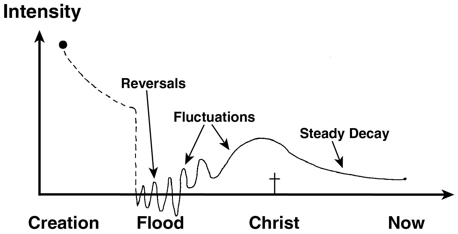
A theoretical model of the earth’s changing magnetic field appeared in our article The earth’s magnetic field: evidence that the earth is young (figure 6). This will no doubt be revised over time, but the main point is that we cannot assume the earth’s magnetic field has always been constant, and the strength of the field controls how much carbon-14 is being formed at any given time. Therefore, we must be careful about drawing grand historical conclusions from carbon dating.

Carbon dating is affected by carbon burial during the Flood

There is another reason why pre-Flood remains have old carbon dates. It has to do with the dramatic reduction from the high antediluvian atmospheric carbon dioxide levels to the modern value. This was due to (1) the burial of masses of organic matter (i.e., most of the pre-Flood biota), (2) the formation of chalk (CaCO₃) deposits from coccolithophore and foraminifera blooms during and after the Flood year, and (3) the revegetation of the earth after the Flood. All these drew down the atmospheric CO₂ to the modern level, which happens to be suboptimal for plant growth. Secular sources tell us that atmospheric CO₂ levels in the early Paleozoic (e.g., pre-Flood) were at least 15 times higher than they are today. Given a constant influx of cosmic rays and the assumption that the amount of carbon-14 is proportional to cosmic ray influx and not the availability of carbon in the atmosphere, this alone is equal to about four half-lives, accounting for over 20,000 years of the inflated pre-Flood carbon dates.

A reduction in atmospheric CO₂ levels would result in a relatively rapid and large increase in the ¹⁴C/¹²C ratio following the Flood, even without the effect of a declining magnetic field. To this we can add volcanic activity, which adds ¹⁴C-depleted CO₂, but we have no idea how much of this there was. Many volcanoes don’t produce much CO₂. Clearly, there was a huge drop in atmospheric CO₂ from the pre-Flood to the post-Flood world, so the amount of volcanic CO₂ contributed during the Flood was either not large or the volcanic CO₂ was absorbed by the formation of limestone. Either way, the effects of the reduced atmospheric CO₂ is going to be large and will occur in a much shorter time frame than the increase in ¹⁴C over time due to a decaying magnetic field.

How far back can you go?

At present, estimated ages of about 50,000 ‘years’ are easily obtainable. This amounts to about 9 half-lives of carbon-14 (½⁹ or ⅟₅₁₂ of the original amount of ¹⁴C). It is possible to measure older dates, but there are no fixed historical events that far back from which we can obtain samples for calibrating the machines. Also, being that so little carbon-14 is left after that much time, any errors in the measurement have a much greater potential effect. For these reasons, archaeologists have shied away from reporting older dates, even though the machines can certainly produce results for these samples.

Interestingly, we have done a lot to throw off the carbon clock in modern times. For example, since coal, oil, and natural gas have less carbon-14 than wood, the burning of fossil fuels during the Industrial Revolution dumped a lot of ‘old’ carbon into the atmosphere. This creates a calibration plateau from 1700 to 1950 that is a bit of an annoyance to carbon dating specialists. Yet, that was nothing compared to what happened in the nuclear age.

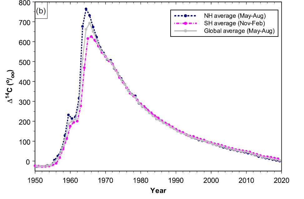
The atmospheric testing of nuclear weapons added a massive amount of carbon-14 to the atmosphere.⁶ This was one of the best things to happen to the carbon dating community, however. The detonation of hundreds of atomic weapons in a short period of time, followed by a sudden cessation when the Partial Nuclear Test Ban treaty went into effect in 1963, produced a “bomb peak” of carbon-14, which has been decaying ever since (figure 7). Samples from 1955 through about 1990 are easily dated with best-ever precision because of the “bomb peak” calibration curve.

Oceanographers have even picked up a plume of modern carbon spreading across the sea floor. Atlantic bottom water is formed at the ice-ocean interface. As ice is formed, salts are excluded. Thus, dense, cold, salty “thermohaline” waters sink to the bottom in the far north. This creates a bottom current of seawater that is slowing flowing southward. You can tell how far the current has travelled since 1950 by simply measuring the carbon-14 content of the water!

How does carbon-14 get from the air into a bone?

Carbon-14 is made in the upper atmosphere. It then combines with oxygen to form CO₂. Winds slowly circulate it everywhere, and it is eventually taken up by plants during photosynthesis. While the plant is alive, the proportion of carbon-14 in the leaves, bark, sugars, and other plant parts essentially (but not exactly) matches the amount in the atmosphere. Animals then eat the plants and the carbon-14 becomes part of the animal. Carnivores eat the herbivores, decomposers consume what the animals leave behind, etc. In this way, Carbon-14 is slowly distributed throughout the biosphere.

Once an animal or plant dies, it is no longer exchanging carbon with the atmosphere. Whatever carbon-14 is included in the wood, bone, or fibers left behind will begin to slowly decay.

How carbon dating is done

The ¹⁴C dating technique involves multiple, complex steps, but it is a fascinating scientific process.

Samples to be analyzed are sent to one of the many carbon-dating laboratories in the world. Technicians visually examine the material under a microscope and manually pick out any odd particles that don’t match the material type. While they are doing this, they confirm that the sample is correctly labeled as bone, cloth, wood, etc.

The second step is to perform a thorough chemical cleaning. This often involves washing with inorganic solvents, acidic solutions, and/or alkaline solutions to remove contaminants like fingerprints, oils, etc. This is very important, considering the controversy about the Shroud of Turin and supposed ‘contamination’ (see below).

In recent years, many laboratories started burning the cleaned sample in an elemental analyzer, which is coupled to the graphitization system. The sample is gassified under high heat in the elemental analyzer. In this way the lab can gain other information about the molecular composition of the sample from the analyzer. The CO₂ is then turned into graphite by reacting with hydrogen at high temperature in the presence of iron powder, which acts as a catalyst.

An older method involved placing the sample in a quartz tube with some copper II oxide (CuO) and silver wire. The air in the tube was evacuated, the tube was sealed, and it was then heated to 900°C overnight. At this point, all the carbon in the sample had been converted into CO₂, using the oxygen from the copper oxide. The silver removed any nitrogen oxides and sulfur oxides produced by the nitrogen and sulfur in the sample. The tube was opened in a closed system of pipes and the CO₂ was collected by cooling it in liquid nitrogen. This was then used to create graphite, as described above.

The cleaned, purified, burned, sometimes liquified, and re-solidified carbon is now ready to be tested. A small amount (typically 0.5–2 mg, about 1,000 times less than older methods required) of the graphite is placed in a sample holder, along with several calibrated carbon standards, and inserted into the front end of a long machine. The air is evacuated from the sample chamber. The graphite is then atomized by hitting it with a high-energy beam of caesium ions.

Caesium is famous for being one of the few metals that are liquid at room temperature.⁸ It is also the easiest metal to ionize.⁹ When the heavy ions strike the carbon source, the surface is blasted into carbon atoms and ions, which are then sent into the detection part of machine.

Detecting carbon-14

There are several different configurations used in radiocarbon labs, and the techniques are constantly being refined. Thus, there is no single explanation of the measurement techniques. However, there is a general approach that most AMS labs share (figure 8).¹⁰

Synal, Jacob, and Suter 2000

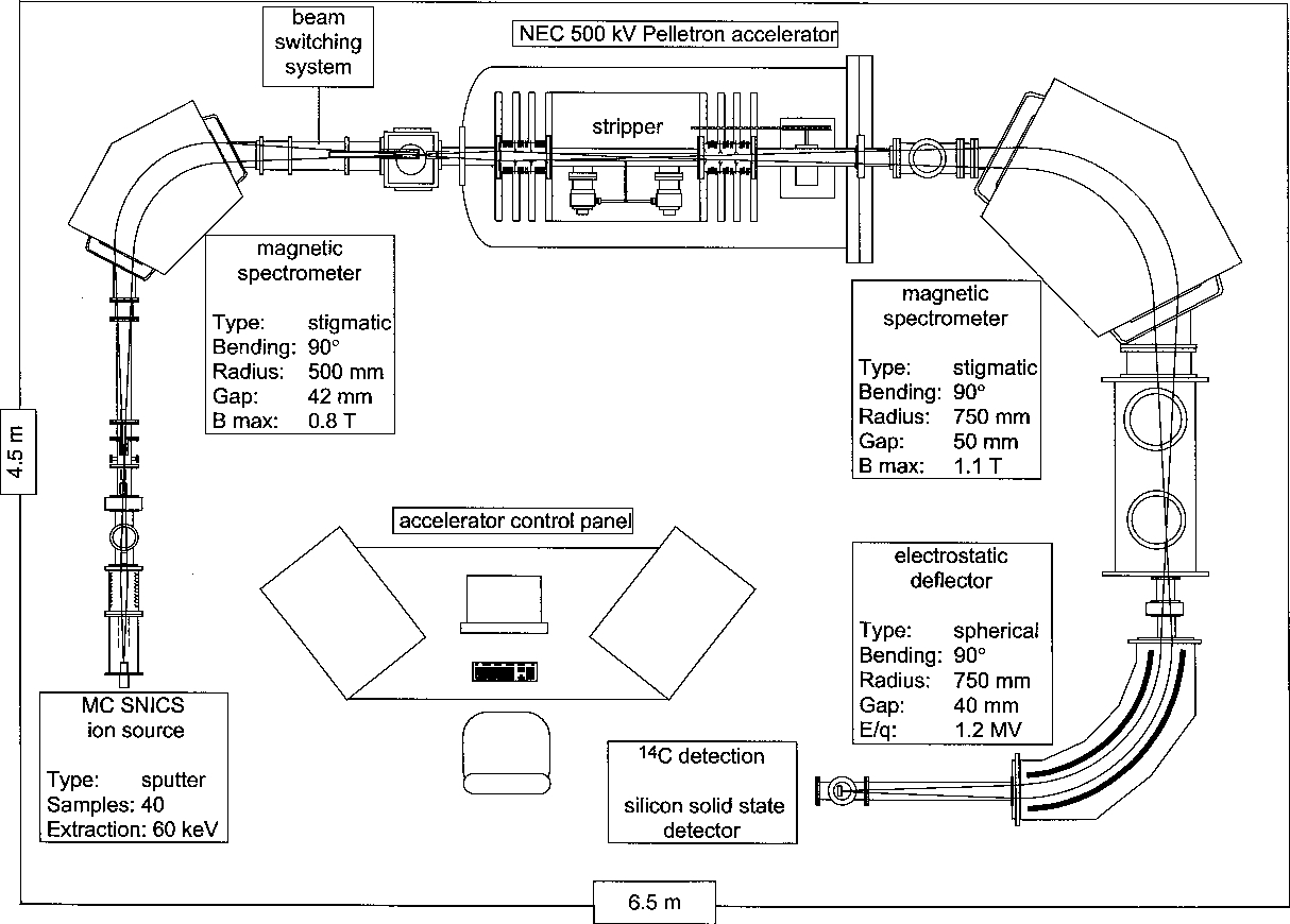
The caesium ions donate electrons to some of the carbon atoms they are striking to form negatively charged carbon ions. A strong (~40 kV) electric field is applied to the chamber, which causes the ions to shoot past a magnet and into an acceleration tube full of argon gas. The argon is a stripper gas, turning the former negative ions into positive ones. Thus, instead of being pulled back toward the magnet, they are now pushed away.

The stream of positively charged carbon ions are then sent down a long tube toward a series of detectors and more strong magnets.

These fast-moving, positively charged ions will produce localized magnetic fields as they move. Thus, if you send one of these ions past a magnet, its path will bend as the two magnetic fields interact.¹¹ By passing the ions past a magnet with just the right strength and angled in just the right direction, you can get the ion beam to turn in a specific direction, but the heavier ions will not bend as much. Thus, the ion beam is separated into distinct ion streams inside the machine.

“Atom smashers” operate on the same principles. For example, at the Large Hadron Supercollider in Europe, propulsion is caused by electric fields. Strong magnets are used to get the charged particles to go in a circle. Linear accelerators also exist. They use oscillating magnetic fields to accelerate charged particles in a specific direction. Accelerator mass spectrometers are a hybrid of these.

The streaming ions are detected with a Faraday cup. This is a simple device that is hooked up to an electric circuit. When an ion strikes the inside of the cup, it creates a small electric current. Importantly, the current is solely based on the charge, and has nothing to do with mass. The circuit must be extremely sensitive and extremely accurate, for even if several billions of ions are striking the detector per second, the current will only be about one nanoamp. An ampere is defined as a current of 1 coulomb of electric charge per second, and a coulomb is 6.241 × 10¹⁸ electric charges. In other words, the current in the circuit can be directly converted into the number of atoms (each with a charge of -1) striking the detector per second.

Here’s where the magic comes in. The carbon ions have the same charge and the same magnetic field strength, so they have the same Lorentz force acting on them. But the ions do not all have the same mass. Since they have different numbers of neutrons, the masses of the three isotopes of carbon are significantly different. ¹³C is 8% heavier and ¹⁴C is 17% heavier than ¹²C. Some AMSs can even differentiate the tiny mass difference between ¹⁴C and ¹⁴N.

As the ions strike each detector, the measurements are sent to a computer. This machine is highly accurate but note that it is not counting individual atoms for the most abundant isotopes. For ¹⁴C, the oldest samples will only generate a few to a few hundred detections in a typical three-minute run, so atoms can absolutely be counted individually. However, the machine is just comparing the amount of current generated in the detectors. It is the ratio of carbon isotopes that is important. This way, it does not matter how much of the sample made it into the beam. One microgram of a sample will have the same relative isotope ratios as one gram of that same sample.

The AMS is orders of magnitude more sensitive and more accurate than the old scintillation counters. Also, the scintillation counters can only measure the atoms that decay. The AMS is measuring all the atoms present.¹²

How much does it cost?

At present, a ‘date’ can be obtained from a radiocarbon lab for about $500 per sample.

Interpreting the data

Carbon dates are usually presented in ‘years before present’ (with the ‘present’ being defined as the year 1950). Sometimes, a date will be converted to AD or BC. Occasionally, you might see a mention of ‘percent modern carbon’ (pmc) or you might also see a phrase like “del ¹³C”. This refers to a complicated ratio of ratios between the ¹³C and ¹²C values of an unknown sample and a standard reference.

Yet, you cannot stick a sample into an AMS and get a ‘date’. Instead, all results must be compared to a known standard, usually several. The goal is to have a standard that is close enough in age that it yields similar values. Operators will generally load sample references that bracket the expected date for the sample. There are reasons why a carbon-14 lab will ask you the expected age of a sample before they run the experiment. It is not like they are deliberately giving you the ‘answer you expect’.

Isotopic fractionation

The results will almost always be corrected for ‘isotopic fractionation’. There are many processes that discriminate among the three carbon isotopes. Since carbon-12 is lighter, it is preferentially used in most biological and chemical reactions. Isotopic fractionation affects how much carbon-14 is absorbed by plants from the atmosphere, by herbivores when they eat the plants, and by carnivores when they eat the herbivores. Thus, a tree branch, a cow bone, and a lion bone from the same date in history will have measurably different carbon ages. We must also account for the differences between land and sea. It takes time for carbon-14 to get into the ocean, and the oceans have a long (~1,000 year) cycle time. Fractionation also affects the rate of carbon-14 penetration into the oceans and how fast it leaves (because it is lighter, ¹²CO₂ evaporates faster). The net effect is that ocean water appears to be about 400 years ‘older’ than the atmosphere. This is known as the marine reservoir effect (MRE), but do not make the mistake of thinking that all ocean water has the same carbon ‘age’. There are significant differences from one place to another, even at the same place at different times.

Isotopic fractionation also affects the carbon dating methods used in the laboratory. Each step (vaporization, liquefaction, solidification, and ionization) involves some degree of isotopic fractionation.

Note, this does not mean that carbon dates are made up. However, it does mean that there is a lot of art to this science. Carbon dating experts must be dedicated to their craft.

After this, the measurement must be calibrated using the standards included in the run and a historical model will be applied to the final results. This is one of the most difficult steps.

For further discussion on the MRE, see the section on Radiocarbon dating in Andrew Sibley’s article on the Kaystros Estuary near Ephesus.

Applying historical models

As stated above, you cannot obtain a carbon date without referencing a known standard, but it is a lot more complicated than simply comparing a known date to an unknown date. The amount of carbon-14 in the atmosphere varies seasonally and latitudinally. It even changes depending on the direction of the wind (i.e., is it coming off the ocean or off the land?).

When building a calibration curve, data might come from tree rings, coral skeletons, cave formations, or laminated lake sediments, but note that these data are associated with many historical assumptions of their own. Even the newest calibration curve, IntCal20, is only a general model and does not include regional differences:

The conclusion drawn there is that there is as yet insufficient information to quantify such effects or indeed to fully understand the contribution from different underlying mechanisms. The potential issues are: different growing seasons for the material dated compared to the calibration datasets, localized addition of CO2 from different reservoirs (such as ocean upwelling, anthropogenic sources, and local volcanic vents), mixture of air masses from both hemispheres in the tropics [reference], and overall trends with latitude or altitude.¹⁴

With the exception of the potential mixing of carbon from different reservoirs, they expect that the seasonal and regional differences will be small, approaching the measurement precision of the machine.

Can a global calibration curve really be applied to material from, say, ancient Egypt? Seasonal winds have a strong effect here, sometimes blowing steadily north, sometimes blowing steadily south, and sometimes not blowing at all. Long-term changes in weather patterns should mean that Southern Europe and Northern Africa need to be treated as separate carbon reservoirs, but we simply do not have the data to do this (yet). This also affects the dating of artifacts in Israel, so these calibration curves are of utmost importance to get right.

Historically, there have been multiple events that should have major effects on carbon-14, but we are unable to measure them at present. For example, at the end of the Ice Age (about 10,000 years before present in the evolutionary dating scheme; about 4,000 years ago in the biblical model) the Mediterranean was a freshwater lake. So much snowmelt was pouring down the tributary rivers in Europe and Asia that it formed a freshwater lens across the entire surface, similar to the situation in the Black Sea today. The deeper saltwater layer was cut off from ready sources of carbon-14. Yet, the Mediterranean is not fresh water today. Sometime in the historical period, well within the abilities of carbon-dating techniques to detect, the Mediterranean turned over. In the evolutionary scenario, this would have dumped a massive amount of ‘old’ carbon into the air and would affect the carbon dates of anything downwind (e.g., Israel and Egypt). This illustrates the tenuous nature of carbon dates. Yes, we can accurately measure the amount of carbon-14 in a sample, but how well this reflects a specific historical time period is debatable.

Known issues with carbon dating

There are multiple issues that complicate the art of carbon dating. Many of these are not usually addressed in public. For example, it is known that trees growing in the vicinity of volcanic areas can often ‘date’ much older than they really are. The reason for this is that any CO₂ coming up from under the ground will have little to no carbon-14. This ‘infinitely old’ carbon will mix with the carbon in the atmosphere, meaning the carbon taken in by the plant will have a false appearance of age. This was first noticed in Italy, but examples of this phenomenon have been documented worldwide.

Carbon dating has also been performed on anomalously old material. This includes wood from the Hawkesbury Sandstone near Sydney, Australia. It was assigned an age of 33,720 ± 430 years bp, with a δ¹³C_PDB value of –24.0‰. That sandstone is supposedly 225–230 million years old. Another piece of wood, from central Queensland, was carbon dated to 37,500 years bp, with a δ¹³C_PDB value of –25.69‰. An adjacent basalt layer, formed from lava that had also charred the wood, was ‘dated’ to 47.5 MA by potassium argon dating.¹⁵ Not only did the δ¹³C results rule out contamination for these wood samples, but the carbon dates are impossible for the evolutionary model. The same can be said of carbon-dates on dinosaur bones (multiple dates, generally ranging from 30–40 thousand years old).¹⁶

Carbon dating has also been applied to coal, from ‘20-million-year-old’ Miocene coal to ‘300-million-year-old’ Pennsylvanian coal. Every coal sample contained carbon-14. They even contained approximately the same amount of carbon-14. There is no way to physically contaminate all the coal in the world with carbon-14. The evidence is that coal is young, because there should not be any carbon-14 left in anything that that is claimed to be millions of years in age.^17,18

“Old” carbon dates do not invalidate the Bible

But do these carbon dates invalidate the biblical timeline? The earth, after all, is only a few thousand years old. Nothing can even be tens of thousands of years old, yet these ancient samples consistently ‘date’ older than is allowed. This is not a problem, because the dates should be strongly constrained by the amount of carbon-14 in the antediluvian world (i.e., little to none). In other words, even if there was zero carbon-14 in this material, it would fit with biblical expectations. Yet, the opposite is not true. Even a little bit of carbon-14 in extremely ‘old’ material is fatal to evolutionary expectations.

Recalibrating carbon dates

What is needed is a way to take the raw carbon dates and recalibrate them according to the biblical timeline. Figure 9 shows a very rough approximation. I pegged the “antediluvian” era to 30,000 carbon years before present (an average of the values seen in dinosaur bones). The date for Abraham is in the range of carbon dates for the Chalcolithic (6,000 YBP), because we know that Abraham, Isaac, and Jacob lived in Beersheba and the latest archaeological evidence for intensive grain cultivation (Genesis 26:12) in the region is from the Chalcolithic (aka, the Copper Age). The red dashed line represents the real historical age. The “present” is defined as the year 1950 (the final data point), but “zero” on the X axis is the year 2022. I used straight lines to connect the blue dots to indicate that this is not a curve that can be represented by a formula. It is a conceptual model only and will be subject to much debate and refinement.

If, as stated above, the earth’s magnetic field strength has been declining by 5% per century, and if the decline has been steady (which is not at all guaranteed), the magnetic field would have been about nine times higher at the time of the Flood, meaning there should have been a lot less carbon-14 in the atmosphere before the Flood. The bomb peak took about 100 years to reach the modern equilibrium, so I assume the concomitant rise in carbon-14 will lag field decay by about a century.

On the other hand, carbon-14 does not have to explicitly follow a simple model of field decay. The magnetic field is only one of several important parameters (e.g., I have discounted the effects of volcanism), and the pre- and post-Flood levels of carbon-14 should not be expected to be the same just because only one year separates them. In fact, the 30,000 YBP measurement for dinosaurs might not be a good measurement for the early post-Flood period at all. It is possible that early post-Flood material could date older than antediluvian samples because of the huge amount of ‘old’ carbon that was dumped into the atmosphere via volcanism.

Counter arguments

Of course, evolutionists have not taken this lying down. They have come up with multiple ways to refute the claims.

“Contamination” is something we consistently hear, but rarely is this contamination documented. “Instrumental errors” are another common refrain, but do they really want to throw their own scientists under the bus? As far as the carbon-14 found in diamonds, we often hear that, yes, there is carbon-14 present, but “uranium” is the cause.^19,20

There are two proposed ways to explain the ‘anomalous’ ¹⁴C in diamonds using uranium. One is cluster decay, where some of the isotopes in the uranium decay chain emit a ¹⁴C nucleus. But this is so rare that the majority of the material in and around the carbon would need to be uranium. We can tell the difference between uranium ore and a diamond, after all. Another way is for the neutrons produced by uranium fission to turn ¹⁴N in the sample into ¹⁴C, in the same reaction that produces radiocarbon in the atmosphere. But in this case, we would expect a strong correlation of ¹⁴C with the nitrogen content of the sample. In fact, it would make the dating unworkable. These arguments go nowhere.

Historical examples

King Richard III

commons.wikimedia.org, Richard Buckley, Mathew Morris, Jo Appleby, Turi King, Deirdre Oullivan, Lin Foxhall

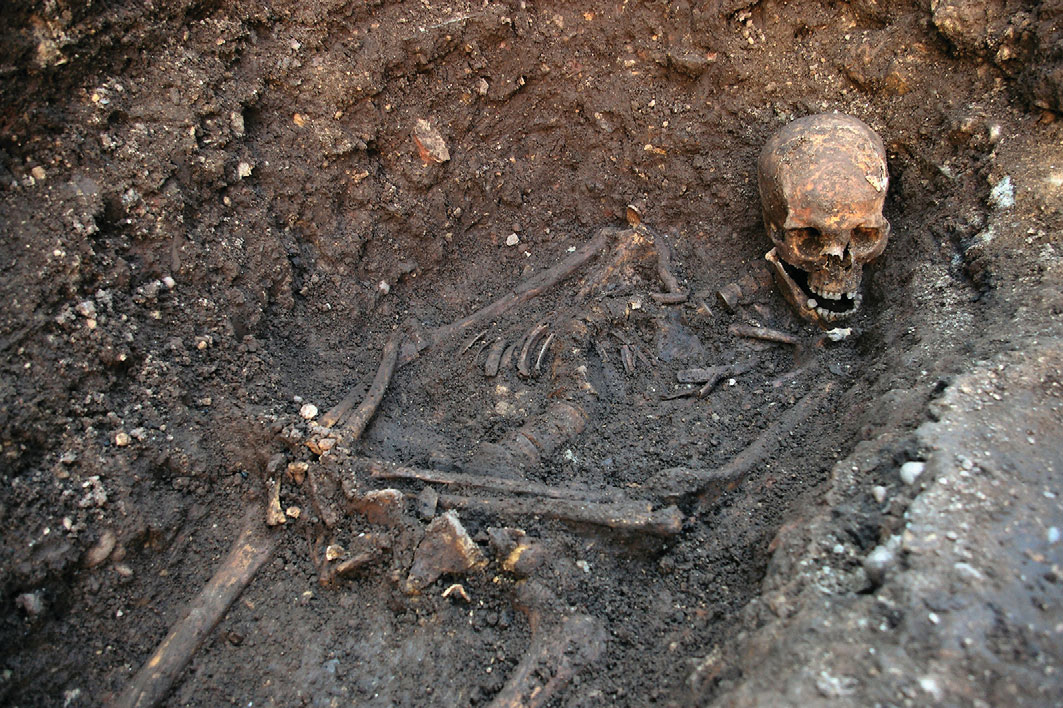
Buried under a carpark not far from CMI’s UK office, the bones of the last Plantagenet King, Richard III (1452–1485) lay in peace. The monastery church where he was hurriedly laid to rest after his death in the Battle of Bosworth Field has long since been forgotten as the growing city of Leicester engulfed the land. Some enterprising historical sleuths realized where his grave should be, and there he was, not near the altar in the Grey Friar’s Priory, but under parking spot ‘R’.

He had an extreme case of scoliosis, mirroring Shakespeare’s claim that he was a hunchback, and they found parasite eggs in the soil around where his innards should have been—parasites that are contracted from eating undercooked beef, and most commoners could not afford that. He has also been stabbed, multiple times, and his skull had been perforated. Clearly, this person died in battle. Every datum was suggesting that this was indeed Richard, except for the carbon date. It was off by decades.

Upon reflection, they realized that, since he was a meat-eating king, they needed to apply a different historical model that they would to a chick-pea–eating peasant. Voilà! His re-dated remains fell right where they should.

This is the state of the art in carbon dating. Yes, it works, but this illustration clearly illustrates that a ‘date’ is not independent from the many assumptions that are used to obtain it.

Syphilis in Europe

A debate has raged for centuries. Did syphilis originate in Europe or in the New World? In other words, did the rapacious Europeans give it to Native Americans or did the Europeans get it from the “Noble Savage” (to use the racist terminology of the era).²¹ It should be easy to resolve the debate, for syphilis is a horrible disease that leaves a person disfigured. In fact, the bones of syphilitic skeletons often have characteristic lesions, as if the bacterium (Treponema pallidum) was turning the person’s skeleton into Swiss cheese, and/or thickened bones. Different strains of T. pallidum cause yaws, bejel, and other diseases of varying severity. It is not always sexually transmitted.

When some syphilitic skeletal remains were discovered in Portugal several years ago, they thought the debate could be settled. The carbon dates placed them prior to 1492. In other words, syphilis was in Europe before the New World was discovered. Some scientists cried foul, however. These people lived on the coast, in a fishing village. They would have eaten a great deal of seafood and, due to the marine reservoir effect, their carbon dates would be skewed downward. They re-calibrated the remains based on a seafood diet and they came out post-1492. Syphilis came from the New World after all?

A few years later, skeletal remains from the 1300s were found under the floor of church in England.²² They had the characteristic lesions of syphilitic patients. Maybe it was a world-wide phenomenon? Or perhaps the disease was brought to England via the Vikings, who had already made contact with the Americas. Further studies have yielded a diverse assemblage of ancient T. pallidum genomes, including ones associated with syphilis, yaws, and bejel from across northern Europe.²³ The carbon dates for these samples are not necessarily post-Columbian, but the diversity of bacterial strains discovered certainly suggests it had been in Europe for a long time. In the end, carbon dating did not help resolve the issue and the question has yet to be answered.

The Shroud of Turin

The Shroud of Turin is a famous medieval artifact that displays a ghostly image of the face and body of a man. This is a controversial subject and not every question about it can be answered here. However, the Shroud was carbon dated in 1988. In fact, four samples were removed and sent to three AMS labs (in the US, UK, and Switzerland) for independent testing. Three control samples were also included: 1) a piece of linen from a Nubian tomb dating to the 11^th–12^th centuries BC, 2) a linen cloth from a mummy of Cleopatra of Thebes from the early second century BC, and 3) threads removed from the cope (a type of coat) of St. Louis d’Anjou from the Basilica of Saint-Maximin, France from the turn of the 13^th century ad. After applying strict calibration methods, the radiocarbon date of the Shroud ranged from 1260 to 1390 AD.

The main counterclaim is that the cloth had been contaminated by modern handling, by soot from medieval candles, by water, and by fire. However, consider what it would take to bring a carbon date forward by thirteen centuries. Datable objects from the time of Christ should have about 78 pMC (percent modern carbon). Items from 1300 AD would have about 92 pMC. At least 1/3 of the sample would have to be ‘contamination’, yet the cloth, even if it is dirty and stained, is clearly the original cloth without massive amounts of clotted wax, soot, or dirt. A second major claim is that the samples were taken from a section of the Shroud that had been repaired. In other words, the material was not original. However, this would require something called ‘invisible reweaving’ with threads that had the same color and texture as material that was more than 1,000 years older. Instead, the ‘repair’, no matter how expertly done, should have been performed by sewing on a patch, and this should be obvious to any careful observer. The sample site has no appearance of being anything but original threads.

We cannot just wish away carbon dating. It is good science. The techniques are sound. Errors can happen, yes, but most of those are easily explainable. Also, the possible dates of the Shroud (e.g., ~33 vs ~1300 AD) are well within the range where we have thousands of other samples that have been dated. The 13-century difference is too much to simply claim ‘error’. Read the main article for further discussion or watch the video.

The destruction of Jericho

Deror_avi, Wikimedia commons

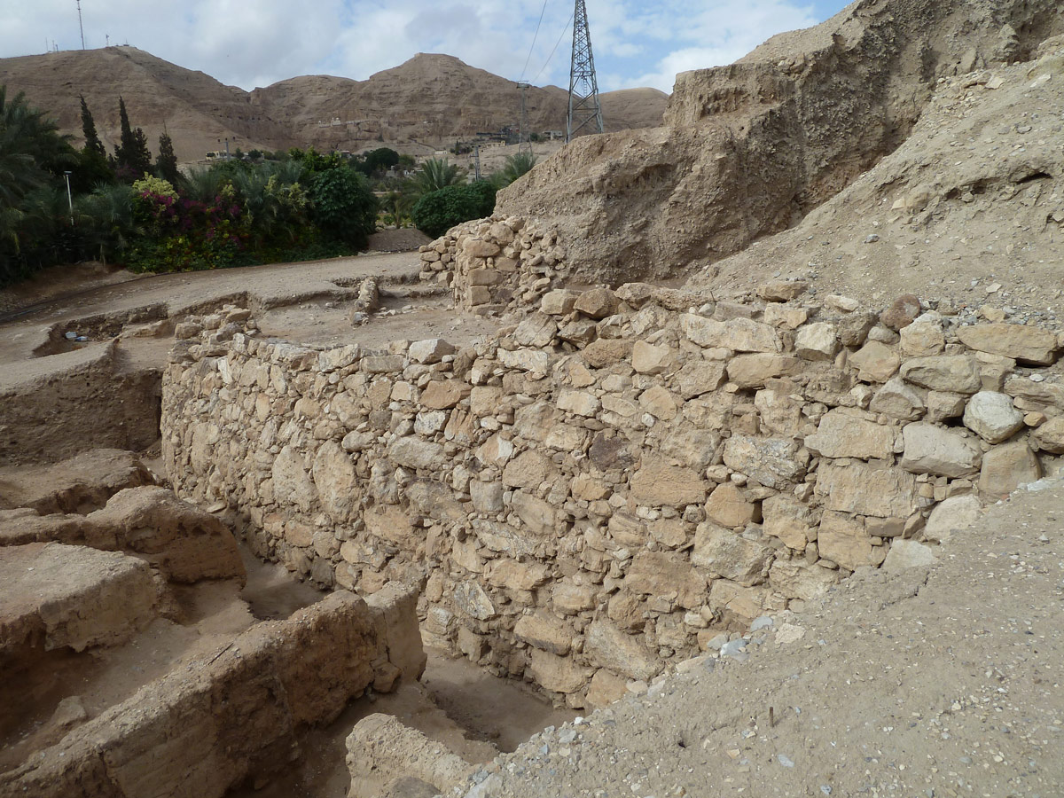
According to the archaeological record, the ancient city of Jericho was destroyed in an unusual way. The walls of the city fell outward, creating a slope that an invading army could easily climb (figure 11). One section of the wall, however, did not fall. Strangely, the city was not looted (at least of food and other non-precious goods) afterward, and it was deliberately burned by fire. With the exception of one small edifice, it was another 500 years before any rebuilding happened at the site. Those are the archaeological details.

Compare the evidence above to the biblical details in the book of Joshua chapters 2 through 6. The Bible claims the walls fell outward, but that Rahab’s house on the wall was still standing (Joshua 2:15–21), that they deliberately burned the city, and that the perishables were left in place, with only gold and silver objects being taken for use in the Tabernacle. Note the curse Joshua laid, “Cursed before the Lord be the man who rises up and rebuilds this city, Jericho. At the cost of his firstborn shall he lay its foundation, and at the cost of his youngest son shall he set up its gates.” (Joshua 6:26). With the exception of a brief occupation by the Moabite king Eglon, which was ended in gruesome fashion by Ehud (Judges 3:12–30), it was not until the time of the idolatrous Israelite King Ahab that Jericho was rebuilt, and Joshua’s curse was fulfilled (1 Kings 16:34).

Everything about ancient Jericho supports the Bible story. Yet, the carbon dates are off by several centuries. Is the Bible in error? No! The carbon dates need to be adjusted.

Egyptian history

Contrary to public opinion, there is no consistent timeline of Egyptian history. They left behind a lot of amazing things (e.g., the pyramids of Giza), but they did not give us many easily datable historical records. The best records for Egyptian history are the king lists of Manetho, who was writing after the time of Alexander the Great. He included many reign lengths and total dynasty lengths, but we don’t have his original writings, only fragments that were recorded by later writers, and these disagree with each other in major ways. There is also a list of kings on the walls of a temple dedicated to Seti I (19th Dynasty) at Abydos. This is an incomplete list, but there are 61 kings listed. Several kings that are left off other lists (e.g., that of Manetho) are included and other kings that we know existed (e.g., Akhenaten, Tutankhamen, Queen Hatshepsut, the Hyksos kings, and others) are skipped. There are also no dates associated with the list of names.

When you examine Egyptian history carefully, you will see well-attested periods interspersed with periods of complete confusion. Some “dynasties” have but a single pharaoh listed; others have an impossible number of pharaohs in a short amount of time. The late periods (e.g., the Ptolemaic and New Kingdom periods) have the most consistent and detailed histories. They also have the greatest number of artefacts that can be carbon dated. The dates are probably off, but not by centuries. Instead, it is the earliest periods where most of the problems lie.

Because of these and other difficulties, Egyptologists turned to carbon dating.^24,25 This gave them a general scheme where the major pieces could be placed in order, but a clear pattern emerged where the carbon dates were consistently older than the dates derived from archaeology.²⁶ This has caused much contention. Carbon dating the most recent periods of Egypt has shown to be relatively accurate to within tens of years to a couple of hundred years from known dates. But carbon dating the older pre-dynastic and Old Kingdom artefacts have shown the greatest discrepancies. As these are from the earliest post-Flood periods, it is expected that they would vary greatly compared to the biblical timeline.

Consider all that was written above. The effects of the Flood and the decaying magnetic field of the earth would combine to magnify carbon dates as one goes back in time. Egypt was clearly settled soon after the Flood, so the dates of the earliest remains would be magnified the most. Currently, a biblical re-calibration curve for carbon dates does not exist so we can only talk in generalities. However, we can accept the general order of the major events in Egyptian history. The earliest events need to be brought forward in time, the middle dates need to be adjusted a little, and the latter dates do not need to change much at all. In fact, carbon dating is very accurate over the last 2,000 years.

Conclusions

Is carbon dating a good argument for biblical creationists? Yes! Carbon dating is a great confirmation that the earth is young. It is an indisputable fact carbon-14 can be found in carbon-containing objects that are claimed to be millions, even billions, of years old. Yet, carbon-14 cannot last that long. Period.

There are challenges, however. Some of those deal with unknown calibration points deep in history, which will be strongly influenced by the after-effects of Noah’s Flood. Other challenges deal with claims of contamination (which is not possible in a diamond), machine error (which would then question all carbon dates), or improbable physical settings (e.g., a diamond that is being bombarded with neutrons from uranium, but no uranium is present in the sample).

We don’t have to reject all carbon-14 dates out of hand, but we do have to carefully weight the strengths and weaknesses of the method. Carbon dating is still a challenge to biblical archaeology and a biblical recalibration curve is desperately needed. On the other hand, we can rest on the fact that ¹⁴C found in diamonds, coal, and dinosaur bones is loudly proclaiming the earth is young and we have good reason to believe the ‘oldest’ carbon dates are artificially inflated due to the events surrounding Noah’s Flood.

Acknowledgements

This article was reviewed by a PhD-level physical chemist (Dr Jonathan Sarfati), a Masters-level Egyptologist (Gavin Cox), a PhD-level archaeologist who specializes in carbon dating, a PhD-level chemist who runs a carbon-dating laboratory, and a PhD university professor in electrical engineering.. This article would not have been possible without their positive criticisms. Any remaining errors are my own.

Related Media

Tree ring dating

References and notes

- You can do this calculation yourself on a spreadsheet or even the calculator function on your phone. Start with 1 × 10⁵⁰ and divide that number by 2 until you get to a number less than 1. Then, multiply 5,700 years by the number of times you divided by 2. I get 957,600 years. See also the calculation in Diamonds: a creationist’s best friend, Ref. 3. Return to text.
- Linick, T.W. et al., Accelerator mass spectrometry: the new revolution in radiocarbon dating, Quaternary International 1:1–6, 1989. Return to text.
- Arnold, J.R. and Libby, W.F. Age determinations by radiocarbon content: checks with samples of known age, Science 110(2869):678–680, 1949. Return to text.
- Morelle, R., New timeline for origin of ancient Egypt, bbc.co.uk/news/science-environment-23947820, 4 Sep 2013. See also Bates, G., Egyptian chronology and the Bible—framing the issues, 2 Sep 2014. Return to text.
- The raw data for the Irish oak tree ring can be found at chrono.qub.ac.uk/bennett/dendro_data/dendro.html, last accessed 14 Mar 2022. Return to text.
- Hua, Q. et al., Atmospheric radiocarbon for the period 1950–2019, Radiocarbon 1–23, 2021. Return to text.
- Carbon also weighs 12.0107 kg/mol, where 1 mol equals the number of atoms in 12 g of carbon-12, or Avogadro’s Number 6.02214 × 10²³ atoms. An AMU is also called a Dalton (Da), after the great creationist chemist John Dalton (1766–1844) who introduced atomic theory into chemistry. Return to text.
- If the room is quite warm—the melting point of caesium is 28.5°C (83.3°F). Return to text.
- In one caesium ion gun, caesium metal is heated to about 150°C. This is well below the boiling point 671°C (1240°F), but enough for some caesium vapour to rise. The vapour rises through a tube, until it hits the ionizer, a hollow tube of molybdenum heated to about 1,300°C. At this temperature, the caesium atom readily gives up an electron to form Cs⁺ ions. They are accelerated by an 8kV voltage towards the graphite. See: Cesium sputter ion source for carbon accelerator mass spectrometry, whoi.edu, accessed 28 Feb 2022. Return to text.
- Synal, H.-A., Jacob, S.A.W., and Suter, M., The PSI/ETH small radiocarbon dating system, Nuclear Instruments & Methods in Physics Research Section B-beam Interactions with Materials and Atoms 172:1–7, 2000. Return to text.
- A magnetic field deflects a moving electric charge in a direction perpendicular both to the field direction and the charge’s direction of movement. The strength is proportional to charge, field strength, and the sine of the angle between them. The magnetic field causes a deflection. An electric field exerts a force on any charge, proportional to charge and to field strength. The combination, the electromagnetic or Lorentz force, is given by F = q(E + v × B).Acceleration is inversely proportional to mass, as per Newton’s Second Law of Motion. Return to text.
- Yet, something strange happened when these machines were first put into use. As a cross-check for contamination AMS labs measure the amount of ¹³C in something called the Pee Dee belemnite (PDB). Belemnites like the famous Belemnitella americana were squid-like animals with 10 tentacles and a hard internal shell. This one came from the Late Cretaceous Peedee formation in North and South Carolina (USA), which evolutionists ‘date’ to at least 66 million years old. That shell, the PDB, was the standard used for calibrating ¹³C/¹²C isotopic ratio measurements across the world for decades. I am still trying to track down the source for this claim, so it is being placed here in a footnote and not in the main text. They were not using the PDB to test for ¹⁴C, yet it has a small but measurable amount of ¹⁴C. In fact, the amount of ¹⁴C is 80 to 100 times above the detection level of the machine. Perhaps it is not as old as they thought! Return to text.
- For ¹⁸O, the isotopic standard is called the Vienna Standard Mean Ocean Water (VSMOW). Return to text.
- van der Plicht, J. et al., Recent developments in calibration for archaeological and environmental samples, Radiocarbon 62(4):1095–1117, 2020. Return to text.
- Snelling, A., Radioactive ‘dating’ in conflict! Fossil wood in ‘ancient’ lava flow yields radiocarbon, Creation 20(1):24–27, 1997. Return to text.
- Thomas, B. and Nelson, V., Radiocarbon in dinosaur and other fossils, CRSQ 51:299–311, 2015. Return to text.
- Giem, P., Carbon-14 content of fossil carbon, Origins 51:6–30, 2001; grisda.org/origins-51006. Return to text.
- Baumgardner, J.R. et al., Measurable ¹⁴C in fossilized organic materials: confirming the young earth creation-flood model, Proc. 5th ICC, pp. 127–142, 2003. Return to text.
- Thomas, B., Contamination claims can’t cancel radiocarbon results, Acts & Facts 49(4), 2020, icr.org. Return to text.
- Cupps, V.R. and Thomas, B., Deep time philosophy impacts radiocarbon measurements, CRSQ 55(4):212–222, 2019. Return to text.
- Woodmorappe, J., The anti-biblical noble savage hypothesis refuted: Do peoples free of biblical influence actually live in harmony with nature and each other? rae.org, accessed 28 Feb 2022. Return to text.
- Hagmann, M., Columbus didn’t do it, science.org/content/article/columbus-didnt-do-it, 31 Jul 2020. Return to text.
- Majander, K. et al. Ancient bacterial genomes reveal a high diversity of Treponema pallidum strains in early modern Europe, Current Biology 30(19):P3788–3803.E10, 2020. Return to text.
- Dee, M. et al., An absolute chronology for early Egypt using radiocarbon dating and Bayesian statistical modelling, Proc. R. Soc. A. 469:20130395, 2013. Return to text.
- Ramsey, C.B. et al., Radiocarbon-based chronology for dynastic Egypt, Science 328(5985):1554–1557, 2010. Return to text.
- Kutschera, W. et al., The chronology of Tell el-Daba: a crucial meeting point of 14C dating, archaeology, and Egyptology in the 2nd millennium BC, Radiocarbon 54(3–4):407–422, 2013. Return to text.
Readers’ comments
Comments are automatically closed 14 days after publication.