

Journal of Creation 35(1):70–77, April 2021
Browse our latest digital issue Subscribe
Ice core oscillations and abrupt climate changes: part 2—Antarctic ice cores
The uniformitarian age of the Antarctic Ice Sheet has increased greatly and is believed to have originated in the Oligocene, based mainly on ice-rafted debris in deep-sea cores. In a debate with Ken Ham, Bill Nye thought that the East Antarctic Ice Sheet could be dated by annual layers to 680,000 years ago. No annual layers are recorded in this ice sheet. The two West Antarctic ice cores were analyzed, which are very similar to the ice cores on Greenland. The newest WAIS (West Antarctic Ice Sheet) Divide ice core did not even show a complete section during the Ice Age. The East Antarctic ice cores, showing what are interpreted to be multiple ice ages, are much different from those on West Antarctica. An isostatic correction was applied to each ice core to determine the elevation of the bedrock at the start of the Ice Age. The East Antarctic ice cores are dated by simply ‘wiggle matching’ to oxygen isotope oscillations in deep-sea cores, which are dated by assuming the astronomical or Milankovitch mechanism of the ‘ice ages’. Millennial-scale oscillations, correlated to deuterium isotope ratios, are also measured in Antarctic ice cores. These ‘abrupt’ climate changes are of small amplitude with a slow rate of change. There are also about ⅓ as many than observed in Greenland ice cores.

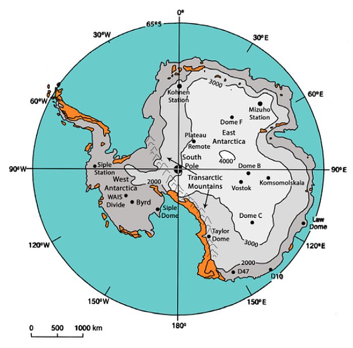
Part 11 analyzed the large-scale and small-scale changes in the oxygen isotope ratios in Greenland ice cores. This ratio is believed to be correlated to temperature, although this is a simplification. The changes are correlated with many other variables, such as various chemicals in the ice, e.g. Ca2+ and Na+, and gases in the ice core bubbles. The small-scale changes, called Dansgaard-Oschger (D-O) or Heinrich events, were assumed to be millennial-scale radical climate oscillations. The abrupt climate changes were believed to take place in a decade to a few years. This second part will focus on the Antarctic ice cores (figure 1), which have similarities and differences to the Greenland ice cores.
The secular view of the origin of the Antarctic Ice Sheet
Within uniformitarian thinking, the age of the Antarctic Ice Sheet has been controversial and has changed with time. It is really two different ice sheets: the West Antarctic Ice Sheet (WAIS), about half of which developed over mountains and the other half developed over the ocean water in between mountains; and the East Antarctic Ice Sheet. At one time, scientists believed that the ice sheet developed in the late Pliocene and/or Pleistocene,2 the general secular ice age period, which makes sense within their paradigm. However, the East Antarctic Ice Sheet is now believed to have started developing in the mid-Cenozoic after the so-called Eocene warm period, about 40 Ma,3 and it reached a steady state at about 15 Ma.4 This radical change to more than 10 times the previous age is based on what is believed to be ice-rafted debris (IRD) from deep-sea cores dated to that time.5 Anti-creationist geologist Arthur Strahler challenges creation scientists:
“Increasing the duration of the Ice Age by a factor of about 10 greatly increases the stress upon the creation scientists, who must compress the events of 15 m.y. into 4,000 y. of post-Flood time.”6
This is a case of stretching out the secular age based on other data sets. Such stretching of events further back in uniformitarian time seems to be typical. The marsupials found in the Riversleigh Park of north-west Queensland were at first dated to the Pleistocene, but with time the age was pushed back into the Miocene and even the Oligocene.7 This was accomplished mainly by the ‘state of evolution’. Pushing the start of the Antarctic Ice Sheet into the Oligocene in no way implies that the Flood/post-Flood boundary is in the Eocene or Oligocene of the early Cenozoic. We cannot take the subdivisions of the Cenozoic as absolute time markers in biblical Earth history. Each area must be evaluated on its own merits. The Flood/post-Flood boundary could be the late Oligocene/Miocene for the marsupials in Australia or the early Pleistocene for the millions of mammals buried in the upper sedimentary rocks of the High Plains of the United States.8
Bill Nye’s mistaken ideas on Antarctic ice cores
In the Ken Ham-Bill Nye debate in 2014, Bill Nye claimed that scientists find 680,000 snow winter-summer layers in some Antarctic ice cores:
“Let’s say we have 680,000 layers of snow ice and 4,000 years since the Great Flood, that would mean we would need 170 winter-summer cycles every year for the last 4,000 years. I mean wouldn’t someone have noticed that? Wow! Wouldn’t someone have noticed that there’s been winter, summer, winter, summer 170 times one year?”9
He seems to think that creation scientists are really stupid, but maybe he should consider that there may be something wrong with his understanding of ice cores. The quote shows that some secular scientists, like Nye, and probably the general public, believe that the Antarctic ice cores totally demolish the short timescale of the Bible. They must believe also that annual layers are laid down on top of the East Antarctic Ice Sheet and that the Antarctic ice cores show annual layers—clear to 680,000 years. Therefore, the Bible is in error and not to be trusted. However, there is much more to the story.10
The top of the East Antarctic Ice Sheet is so high that it is claimed that only about 5 cm of ice equivalent in snow falls each year11—much too small for annual layers.12 Moreover, there are other complications with any presumed orderly accumulation of each year’s layer of snow. The snow blows around on top of and on the edges of the ice sheet, so there is much mixing of snow from many years. Glaciologists certainly do not date the cores by counting annual layers as implied by Bill Nye; there are no annual layers in the East Antarctic Ice Sheet! Nye was completely ignorant of the situation.
The deuterium isotope ratio
The deuterium isotope ratio, instead of the oxygen isotope ratio, is mostly plotted with depth in Antarctic ice cores. This is the ratio of the amount of deuterium, with one proton and one neutron in the nucleus of the hydrogen atom, divided by the amount of the hydrogen atom, with just one proton in the nucleus. The deuterium isotope ratio is:
δD = [(D/H)sample – (D/H)standard]/(D/H)standard × 1000‰
where ‘D’ is deuterium, ‘H’ is hydrogen, and δD is measured in per mil, i.e. parts per thousand (‰). Because fractionation of isotopes is proportional to molecular weight, the deuterium isotope ratio changes eight times as fast as the oxygen isotope ratio during evaporation of water. The relationship between the two isotope ratios is expressed by the equation:
δ18O = 8δD + d
where ‘d’ is called the deuterium excess, which averages 10‰. The deuterium excess can vary around its average value depending upon a number of variables that are related to the moisture source.

The West Antarctic ice cores
First, we will delve into the dating of the West Antarctic ice cores. There are a number of coastal cores, but these are too difficult to interpret.13 Besides, their timescales are much shorter than those assigned to the central cores and, therefore, are not a big challenge to the creation-science timescale. The Byrd ice core (figure 1) was the second ice core recovered after the Camp Century core in north-west Greenland. It was drilled from 1,530 m above sea level (asl) and reached the bedrock at 2,164 m deep, which is 634 m below present sea level. Figure 2 shows the oxygen and deuterium isotope ratios for this core, with depth on the left and the stretched-out uniformitarian timescale on the right. The top of the core has an annual layer thickness of about 13 cm/yr, thought too thin for annual layers to be visually discerned, since the layers thin with depth. The Ice Age portion of the core is located about 1,300 m down the core, identified by the lower isotope ratios.
A second, long core was drilled on a ridge along the ice sheet divide between ice flowing toward the Ross Sea and the ice flowing toward the Weddell Sea (figure 1). It is called WAIS Divide. It was drilled from the top of the ice at 1,766 m asl down 3,405 m. It was stopped 50 m from the bottom, which means that the core was drilled to 1,639 m below sea level with bedrock at 1,689 m below sea level. However, the ice core reached down only about half way into the Ice Age and was dated to only 68 ka in the uniformitarian timescale. Because of an annual layer accumulation of ice on WAIS Divide of 22 cm, annual layers actually can be determined at the top of this ice core, like in Greenland. Similar to the GISP2 ice core, annual layer counting becomes difficult the deeper in the core, especially since uniformitarian scientists believe the accumulation rate dropped off 50% in the Ice Age (figure 3).15,16 Uniformitarian scientists simply assume that the accumulation rate is proportional to the temperature, based on deuterium isotope ratios. In fact, the annual layer counting stopped at 31 ka, less than half the total time claimed for the ice core. The annual layers must have been difficult to figure between 15 ka and 31 ka with accumulation assumed to be only 11 cm/yr.

The annual layer counting, whether for WAIS Divide or Greenland, starts with a first guess of the number of annual layers based on assumed equilibrium for millions of years. The flow models take this equilibrium into consideration, which is why the annual layers are believed to thin drastically with depth (see part 1, figure 2).1 The flow models are also anchored by various tie points of ‘known’ age with deep time built in. The WAIS Divide ice core even had a ‘tie point’ from a speleothem in the European Alps!15 Thus, the annual layer counting is very subjective with old age built in.
The section of the core from 31 to 68 ka was simply dated by flow modelling and tie points, and it was matched with the Greenland methane record. This correlation is probably good for finding a common timescale for the hemispheres. Methane mixes relatively fast between the hemispheres, and the ice accumulation generally records the atmospheric methane concentration at the time of accumulation. The same cannot be said for CO2 since reactions with dust can change the CO2 in the bubbles (see below). Other tie points came from ‘refined’ oxygen isotope ratios from speleothems from the Hulu cave, China!17
The East Antarctic ice cores
The deep ice cores on East Antarctica (figure 1) are much different from those on West Antarctica and Greenland. The East Antarctic Ice Sheet developed mostly over land, some of it is mountainous, and near the South Pole. Whereas the West Antarctic ice cores show only one ice age or just part of one ice age (the WAIS Divide ice core), uniformitarian scientists claim the East Antarctic ice cores indicate multiple ice ages, as shown by large changes in the deuterium isotope ratios. How could the East Antarctic ice cores be so different from the West Antarctic and Greenland ice cores? This will be answered in part 3.18
Figure 4 shows a comparison between the two main East Antarctic ice cores, Dome C and Vostok, according to depth and according to the stretched out uniformitarian timescale. Dome C was drilled from 3,233 m asl down to 3,260 m, stopping 15 m from bedrock.19 The bottom 60 m was deformed. Therefore, bedrock below Dome C is 3,275 m below the surface at Dome C and 42 m below sea level.

The calculation of ice thickness and isostatic correction for Vostok is tricky. Vostok was drilled from 3,488 m asl and the core reached 3,623 m.20 It was stopped 120 m above the top of the large, deep, subglacial Lake Vostok, which is about 600 m deep, 230 km long, and 50 km wide. The surface of Lake Vostok is currently about 255 m below sea level. When the ice was first building on Vostok, the lake was frozen at the top, but the weight of the ice would have pushed the ice all the way to bedrock. So, for an isostatic correction, the depth of Lake Vostok, 610 m at this location, must be included. So, adding up the height of the ice sheet above sea (3,488 m), adding the depth below sea level of Lake Vostok (–255 m), and the depth of lake Vostok (610 m) yields a total ice thickness of 4,353 m before the ice melted to form Lake Vostok. Six oscillations are claimed for Dome C from the 1,700 m to the 3,200 m level, while only three are claimed for Vostok from 1,800 m to 3,400 m. The bottom four oscillations of Dome C are of low deuterium isotope amplitude with oscillations between ‘interglacials’ that are almost as high in amplitude.21 These glacial/interglacial oscillations are not convincing.

Two other deep ice cores have been drilled on Antarctica. Dome Fuji or Dome F was drilled by the Japanese from 3,810 m asl down to 2,503 m depth in 1995/96 with an ice thickness of 3,028 m (placing the bedrock at 782 asl) (figure 5).22 The core stopped 525 m from the bedrock. The scientists found three glacial and four interglacial oscillations down to 2,503 m, dated at 340 ka. Between 2003 and 2007, a second, deep ice core reached 3,035 m to near bedrock, the bottom of which was dated at 720 ka.23 The large-scale oscillations are very similar to those of Dome C and Vostok.
A fourth deep ice core was drilled at Kohnen Station (Dronning Maud Land), along the downward slope of the East Antarctic Ice Sheet (figure 1). It was drilled from 2,882 m asl and reached 2,417 m deep, the bottom dated at 150 ka and showing one glacial cycle and two interglacial cycles.25 It was stopped 350 m short of bedrock, 115 m asl, because the ice became deformed further down.26 Being closer to the edge of the ice sheet, the ice is moving faster, and it is not surprising that the bottom 350 m is deformed.
Isostasy considerations before glaciation
As with the Greenland ice cores, we must determine the bedrock elevation before glaciation to determine the start of glaciation. This is likely a crucial variable in explaining the East Antarctic ice cores. Table 1 presents the current altitude, ice thickness, present bedrock elevation, isostatic correction, and height of the bedrock at the beginning of the Ice Age.
The ice cores from West and East Antarctic can likely be explained by the elevation of the land at the start of the Ice Age, the time it took for the ice to start accumulating, and the ice accumulation rate.
The West Antarctic Ice Sheet would first develop in the mountains, spread to lower altitudes, and then spread over the ocean water between the mountains as ice shelves. Thickening ice shelves from snow accumulation pushed the ice all the way down to the bottom of the ocean expelling the water (see below). Due to the weight of the ice pushing down the land, most of the West Antarctic land surface now sits below sea level. Considering isostasy, the bedrock of the Byrd ice core, now at 614 m below sea level, would have started about 100 m above sea level. Therefore, the Byrd ice core likely did not start accumulating ice until mountain glaciation extended to the lowlands. Thus, the Byrd ice core likely did not develop until about 200 years after the Flood, which likely is why it is similar to the Greenland ice cores.
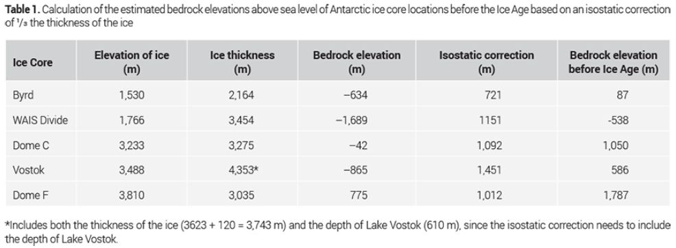
The bedrock on WAIS Divide, on the other hand, is now 1,689 m below sea level. If we add uplift for isostatic rebound, then this ice core started developing at about 550 m below sea level. In this case, the ice must spread not only from the mountains to the lowlands, but also spread as thickening ice shelves over the ocean water between mountains. This would take more time for glaciation to start at WAIS Divide than at Byrd, maybe in about 300 years after the Flood. This would explain why the WAIS Divide ice core starts toward the middle of the Ice Age. It also explains why no previous ice ages or the warm period before the Ice Age show up at the bottom of the ice core.
If we raise the land of East Antarctica for the time right after the Flood, we would have to raise the bedrock of Dome C to 1,050 m and Vostok to 586 m above sea level (table 1). Based on isostatic recovery, the ice of Dome Fuji would start quite high at about 1,787 m asl. Thus, the higher elevations of East Antarctica would likely have started glaciating within about 50 years with cirques in the mountains.
Dating East Antarctic ice cores
Since uniformitarian scientists cannot use annual layer counting, how do they date the East Antarctic ice cores? They use ‘flow modelling’ with the uniformitarian assumptions built in.27 Various ‘tie points’ that have been previously ‘dated’, such as volcanic signals or glacial/interglacial oscillations, are used to anchor the flow models. They also compare each long ice core to those ice cores already drilled and use wiggle matching,45 which seems to be okay since the deuterium isotope ratios are consistent throughout the whole East Antarctic Ice Sheet.
The East Antarctic ice cores, as well as many other Quaternary data sets, are ultimately dated by assuming the Milankovitch or astronomical theory of ice ages in which glacial/interglacial oscillations repeat every 100,000 years for the ‘past’ one million years. The Milankovitch theory is built into flow models and the ‘dates’ of the ‘tie points’. So, the dating of the East Antarctic ice cores is simply done by ‘wiggle matching’ the oxygen isotope ratio, mostly in foraminifera, in deep-sea cores.28 But this wiggle matching assumes the astronomical theory:
“Wiggle matching to existing ice core time scales or orbitally tuned [to the astronomical theory] marine records has often been used as a first indication of the age of an ice core, especially for Antarctic ice cores reaching half a million years and more back in time.”29
Waelbroeck et al. also inform us that they matched (tuned) an earlier Vostok ice core, which showed two large oscillations, to deep-sea cores:
“Taking advantage of the fact that the Vostok deuterium (δD) record now covers almost two entire climate cycles, we have applied the orbital tuning [Milankovitch cycles] approach to derive an age-depth relation for the Vostok ice core, which is consistent with the SPECMAP marine time scale [from deep-sea cores].”30
The SPECMAP marine timescale was earlier tuned to the Milankovitch orbital changes:45
“The deep-sea core chronology developed using the concept of ‘orbital tuning’ or SPECMAP chronology [and] … is now generally accepted in the ocean sediment scientific community.”31
Nothing has changed over the years. This procedure is circular reasoning. Ice cores, deep-sea cores, and other climatic data sets ultimately all assume the Milankovitch mechanism has been ‘proven’, and that this mechanism is data that strongly influences all climatic data sets. This is also why they can claim there were about 50 ice ages of various intensities during the 2.6 Ma of the Quaternary,32 based on about 50 Pleistocene wiggles in a composite ‘stack’ of 57 Milankovitch-tuned deep-sea cores.33
However, the 100,000-year Milankovitch eccentricity cycle is very weak, affecting solar radiation extremely little.34 Moreover, because the uniformitarian scientists changed the date of the Bruhnes/Matuyama normal/reverse transition from 700 ka to 780 ka, the deep-sea core cycles no longer line up with the Milankovitch cycles.35,36 Therefore, the Milankovitch mechanism, thought ‘proven’ in 1976 and to be the ‘pacemaker of the ice ages’,37 is not proven at all. The secular scientists attempted to quietly rescue the pacemaker paper in 1997, but their efforts are not convincing because of selection bias and a capricious handling of the seafloor sediment data.38 All climatic data sets that are fitted to this theory are flawed. Ironically, thousands of papers dealing with climatic data sets as well as pre-Pleistocene sediments have a wrong assumption.39 This means that deep-sea cores and deep East Antarctic ice cores are misdated, even by secular reckoning.
Deuterium isotope ratio correlated to many other variables

The deuterium isotope ratios of the Antarctic ice cores are correlated with many other variables, similar to the situation with the Greenland ice cores. Figure 6 shows the Vostok ice core with four claimed glacial/interglacial cycles that are highly correlated to CO2 with an amplitude of about 100 ppm. However, the CO2 amplitude was about 30% smaller at Dome C than at Vostok.40 Moreover, there are big CO2 differences between Antarctic and Greenland ice cores, which likely is due to chemical effects with dust and acids.41 We cannot trust CO2 from the ice cores to correlate between the hemispheres.
The amount of dust is also correlated with the deuterium isotope ratios in Dome C. However, there seems to be little actual dust in the core, and the ‘dust’ (which is actually volcanic ash) decreases down the core.42 Narcisi et al., state:
“The Dome C ice is generally very clear and the core contains less than twenty visible dust layers. The majority of these layers occur in the uppermost 2200 m and are composed of airborne volcanic ash produced by explosive eruptions.”43
Methane, with a maximum amplitude of around 450 ppbv, is highly correlated with deuterium isotope ratios.21 Seventy-four methane jumps occur in 800 ka, with an apparent rapid increase to the higher values and falling off slowly.44 Non-sea salt Ca, representing continental sources, and sea salt Na from the ocean are correlated with deuterium isotopes.45
Millennial-scale changes
Abrupt climate changes are claimed in the Antarctic ice cores. They are called AIMs (Antarctic Isotope Maximums), but they represent warming of only 1–3°C, much less than those claimed for the Greenland ice cores. Moreover, these smaller-amplitude oscillations do not show an abrupt rate of change, but a more gradual change. The last oscillation before the Holocene is the Antarctic Cold Reversal (ACR). It is questionable whether AIMs can be considered abrupt climate changes.

Furthermore, there appear to be only about 7–9 AIMs in the West Antarctic and East Antarctic Ice Sheets, about ⅓ the number of D-O events in Greenland ice cores (figure 7). Of course, there are numerous other fluctuations of amplitude less than about 1°C, and uniformitarian scientists attempt to also correlate these small fluctuations to D-O events. The average isotope ratio of the seven AIMs decrease up core, probably representing cooling with time, until the Last Glacial Maximum (LGM) was reached.
Conclusions
The Antarctic Ice sheet is now believed to have started about 34 million years ago and reached equilibrium about 15 million years ago. This does not mean all rocks classified as Cenozoic are post-Flood; it depends on how uniformitarians have done their classification. Although Bill Nye claimed in his famous debate with Ken Ham that secular scientists have counted 680,000 annual layers in the East Antarctic Ice Sheet, there are no annual layers in that ice sheet. The two ice cores drilled on the West Antarctic Ice Sheet are very similar to those on Greenland, the newer WAIS Divide ice core not even recording a full glacial cycle. The ice cores on the East Antarctic Ice Sheet are much different, showing up to eight ice ages through the cores to near the bedrock, based on large deuterium isotope fluctuations. However, all ice cores are dated by flow modelling, using ‘tie’ points, dated from other data sets of ‘known’ age. This is how deep time enters into ice core dating. But ultimately, the East Antarctic ice cores are dated by wiggle matching to each other and to deep-sea cores. The latter have been dated by assuming the 100,000 ka Milankovitch cycle. Unfortunately for secular scientists, this Milankovitch oscillation changes the solar radiation distribution on Earth extremely little. There is no forcing for climate change. The Antarctic ice cores show what are interpreted to be millennial-scale oscillations that are correlated to many other variables. However, these so-called abrupt climate changes amount to only 1–3°C oscillations, and there are about ⅓ of them as observed in Greenland ice cores.
Part 318 will show how the large-scale, isotopic ratio oscillations and all the correlated variables in the all the ice cores can be explained within the biblical Ice Age model. Part 447 will provide an explanation for the millennial-scale oscillations and their correlated variables. Part 548 will delve into the mystery of the green, wet Sahara Desert that occurred after Northern Hemisphere glaciation.
References and notes
- Oard, M.J., Ice core oscillations and abrupt climate changes: part 1—Greenland ice cores, J. Creation 34(3):99–108, 2020. Return to text.
- Rutford, R.H. et al., Late Tertiary glaciation and sea level changes in Antarctica, Palaeogeogrphy, Palaeoclimatology, Palaeoecology 5:15–39, 1968. Return to text.
- Barrett, P., Cooling a continent, Nature 421:221–223, 2003. Return to text.
- Anderson, I., A glimpse of the green hills of Antarctica, New Scientist 111(1515):22, 1986. Return to text.
- Crowell, J.C., Pre-Mesozoic ice ages: their bearing on understanding the climate system, GSA Memoir 192, Geological Society of America, Boulder, CO, 1999. Return to text.
- Strahler, A.N., Science and Earth History: The evolution/creation controversy, Prometheus Books, Buffalo, NY, p. 254, 1987. Return to text.
- Archer, M. et al., Riversleigh: The story of animals in ancient rainforests in inland Australia, Reed books, Chatswood, Australia, 1991. Return to text.
- Oard, M.J., Relating the Lava Creek ash to the post-Flood boundary, J. Creation 28(1):104–113, 2014. Return to text.
- Ham, K. and Hodge, B., Inside the Nye Ham Debate: Revealing truths from the worldview clash of the century, Master Books, Green Forest, AR, p. 315, 2014. Return to text.
- Oard, M.J., The Frozen Record: Examining the ice core history of the Greenland and Antarctic Ice Sheets, Institute for Creation Research, Dallas, TX, 2005 (available from ICR by print on demand). Return to text.
- Rafferty, J.P. (Ed.), The Great Ice Sheets, Encyclopaedia Britannica, britannica.com/science/glacier/The-great-ice-sheets, accessed 6 August 2020. Return to text.
- Basille, I. et al., Volcanic layers in Antarctic (Vostok) ice cores: source identification and atmospheric implications, J. Geophysical Research 106(D23):31915–31931, 2001. Return to text.
- WAIS Divide project members, Onset of deglacial warming in West Antarctica driven by local orbital forcing, Nature 500:440–444, 2013. Return to text.
- Gow, A.J. et al., Climatological implications of stable isotope variations in deep ice cores from Byrd Station, Antarctica; in: Black, R.F., Goldthwait, R.P., and Willman, H.B. (Eds.), The Wisconsinan Stage, GSA Memoir 136, Geological Society of America, Boulder, Co, pp. 323–326, 1973. Return to text.
- Sigl, M. et al., The WAIS Divide deep ice core WD2014 chronology – part 2: annual-layer counting (0–31 ka BP), Climate of the Past 12:769–786, 2016. Return to text.
- Fudge, T.J. et al., Variable relationship between accumulation and temperature in West Antarctica for the past 31,000 years, Geophysical Research Letters 43:3795–3803, 2016. Return to text.
- Buizert, C. et al., The WAIS Divide deep ice core WD2014 chronology – part 1: methane synchronizations (68–31 ka BP) and the gas age–ice age difference, Climate of the Past 11:153–173, 2015. Return to text.
- Oard, M.J., Ice core oscillations and abrupt climate changes: part 3—Large-scale oscillations within biblical earth history, J. Creation (in press). Return to text.
- Jouzel, J. et al., Orbital and millennial Antarctic climate variability over the past 800,000 years, Science 317:793–796, 2007. Return to text.
- Petit, J.R. et al., Climate and atmospheric history of the past 420,000 years from the Vostok ice core, Antarctica, Nature 399:429–436, 1999. Return to text.
- Brook, E., Windows on the greenhouse, Nature 453:291–292, 2008. Return to text.
- Watanabe, O. et al., The paleoclimate record in the ice core at Dome Fuji station, East Antarctica, Annals of Glaciology 29:176–178, 1999. Return to text.
- Motoyama, H., The second deep ice coring project at Dome Fuji, Antarctica, Scientific Drilling 5:41–43, 2007. Return to text.
- Watanabe et al., ref. 22, p. 177. Return to text.
- Ruth, U. et al., ‘EDML1’: a chronology for the EPICA deep ice core from Dronning Maud Land, Antarctica, over the last 150,000 years, Climate of the Past 3:475–484, 2007. Return to text.
- Fischer, H. et al., Reconstruction of millennial changes in dust emission, transport and regional sea ice coverage using the deep EPICA ice cores from the Atlantic and Indian Ocean sector of Antarctica, Earth and Planetary Science Letters 260:340–354, 2007. Return to text.
- Dreyfus, G.B. et al., An ice core perspective on the age of the Matuyama-Brunhes boundary, Earth and Planetary Science Letters 274:151–156, 2008. Return to text.
- Schulz, M., On the 1470-year pacing of Dansgaard-Oeschger warm events, Paleoceanography 17(4):1–10, 2002. Return to text.
- Andersen, K.K. et al., The Greenland ice core chronology 2005, 15–42 ka. Part 1: constructing the time scale, Quaternary Science Reviews 25:3246, 2006. Return to text.
- Waelbroeck, C. et al., A comparison of the Vostok ice deuterium record and series from Southern Ocean core MD 88–770 over the last two glacial-interglacial cycles, Climate Dynamics 12:113–123, 1995; p. 113. Return to text.
- Waelbroeck et al., ref. 30, pp. 113–114. Return to text.
- Walker, M. and Lowe, J., Quaternary science 2007: a 50-year retrospective, J. Geological Society London 164:1073–1092, 2007. Return to text.
- Lisiecki, L.E. and Raymo, M.E., A Pliocene-Pleistocene stack of 57 globally distributed benthic D18O records, Paleoceanography 20(PA1003), 2005. Return to text.
- Oard, M.J., The 100,000-year Milankovitch cycle of ice ages challenged, J. Creation 12(1):9–10, 1998. Return to text.
- Hebert, J., A broken climate pacemaker?—part 1, J. Creation 31(1):88–98, 2017. Return to text.
- Hebert, J., A broken climate pacemaker?—part 2, J. Creation 31(1):104–110, 2017. Return to text.
- Hays, J.D. et al., Variations in the earth’s orbit: pacemaker of the ice ages, Science 194:1121–1132, 1976. Return to text.
- Hebert, J., Have uniformitarians rescued the ‘Pacemaker of the Ice Ages’ paper? J. Creation 33(1):102–109. Return to text.
- Oard, M.J. and Reed, J.K., Cyclostratigraphy and Astrochronology, part IV: Is the Pre-Pleistocene Sedimentary Record Defined by Orbitally-Forced Cycles? CRSQ (in press). Return to text.
- Luthi, D. et al., High-resolution carbon dioxide concentration record 650,000—800,000 years before present, Nature 453:379–382, 2008. Return to text.
- Anklin, M. et al., CO2 record between 40 and 8 kyr B.P. from the Greenland Ice Core Project ice core, J. Geophysical Research 102(C12):26539–26545, 1997. Return to text.
- EPICA community members, Eight glacial cycles from an Antarctic ice core, Nature 429:623–628, 2004. Return to text.
- Narcisi, B. et al., First discovery of meteoritic events in deep Antarctic (EPICA Dome C) ice cores, Geophysical Research Letters 34(L15502):1–5, 2007. Return to text.
- Loulergue, L. et al., Orbital and millennial-scale features of atmospheric CH4 over the past 800,000 years, Nature 453:383–386, 2008. Return to text.
- Parrenin, F. et al., The EDC3 chronology for the EPICA Dome C ice core, Climate of the Past 3:485–497, 2007. Return to text.
- Jouzel, J. et al., Orbital and millennial Antarctic climate variability over the past 800,000 years, Science 317:793–796, 2007; p. 794. Return to text.
- Oard, M.J., Ice core oscillations and abrupt climate changes: part 4—Abrupt changes better explained by the Ice Age, J. Creation (in press). Return to text.
- Oard, M.J., Ice core oscillations and abrupt climate changes: part 5—The early Holocene Green Sahara, J. Creation (in press). Return to text.

Readers’ comments
Comments are automatically closed 14 days after publication.